Note that the primary goal of the model is not to make predictions (although it certainly could) but to learn about feature importance, i.e. the interpretation. That choice drives nearly every decision below.
There is a lot of ground to cover from earning an online (however advanced) data science certificate to building your first model for a real use case. The use case here was a customer referral programme at a digital wealth manager, and the question was who refers: which client characteristics predict whether someone brings in another client. This note covers the three major learnings that helped me eventually obtain a performant and explainable model: class balancing, encoding different categorical features, and adopting leakage-proof pipeline.
Class Imbalance
The False vs. True counts of the binary target variable is about 83:17 in the data. This is not hopeless but needs to be addressed. In my first run I did not do so, because I thought the underlying sample size is big enough and the minor class is still large in absolute terms. Then the test AUC score dropped significantly from the training score, and there is the tell-tale sign of class imbalance: high accuracy coupled with a very low recall. This means that the model performs well most of the time on the majority cases and has learned practically nothing from the minority class (the ones evaluated True), hence the high false-negative rate reflected in the low recall.
Before moving on to more aggressive measures such as downsampling or oversampling, we should try scaling the positive weight by using the scale_pos_weight parameter:
from xgboost import XGBClassifier
# Address the class imbalance by scaling the positive weight
scale = (y == False).sum() / (y == True).sum()
XGBClassifier(random_state=42, scale_pos_weight = scale,
              eval_metric='logloss', objective='binary:logistic')
Split training and test set using the stratify parameter:
X_train, X_test, y_train, y_test = train_test_split(X, y,
    test_size=0.2, random_state=42, stratify=y)
As a cross-validation strategy, use StratifiedKFold to preserve class balance across folds, which matters for imbalanced targets:
from sklearn.model_selection import StratifiedKFold
cv = StratifiedKFold(n_splits=5, shuffle=True, random_state=42)
The test AUC score improved significantly and is now closer to the training score after handling the imbalance. The trade-off here is that the model precision dropped significantly in favour of recall, since we now predict more false positives. On the held-out test set that landed at recall 0.71 against precision 0.36: the model catches roughly seven referrers in ten, and is wrong about two-thirds of the clients it flags. Loop back to the business context to determine whether the trade-off is acceptable, or even desired. In my use case it was beneficial to trade a higher false positive for a lower false negative. The cost of surfacing a client who turns out not to refer is a wasted nudge, while the cost of missing one is a referral that never happens.
One further consequence is easy to miss: by reweighting the minority class during training, scale_pos_weight also breaks the calibration of the predicted probabilities. They come out systematically inflated towards the positive class, so a predict_proba output of 0.6 no longer means “a 60% chance this client refers”. That's not an issue if you only ever use the ranking (which is all ROC-AUC reads, and all SHAP needs to attribute contributions). But the moment someone downstream wants to read a score as a probability, or set a threshold from an expected-value calculation, it has to be calibrated first.
Encoding Categorical Features
Boolean Feature
Map True and False to the integer 1 and 0, respectively, for Boolean features. Handling conversions explicitly is always better than implicitly.
# Convert boolean to int
bool_list = ['bool_column1', 'bool_column2']
for column in bool_list:
    df[column] = df[column].astype(np.int32)
Ordinal Feature
Obviously OrdinalEncoder is our friend here. One thing to keep in mind is that the sequence needs to be given explicitly, as the encoder knows nothing of your business logic and will simply put items in alphabetic order, which will invariably lead to headaches at the model-explanation stage.
from sklearn.preprocessing import OrdinalEncoder
enc = OrdinalEncoder(categories = [['LOW_RISK', 'MEDIUM_RISK', 'HIGH_RISK']],
                     dtype=np.int32)
df['risk_expectation'] = enc.fit_transform(df[['risk_expectation']])
Categorical Feature without Intrinsic Order
If there are just a handful of labels in the categorical feature, we should first consider one-hot encoding:
df = pd.get_dummies(df, columns=['feature_1', 'feature_2'],
                    drop_first=True, dtype=np.int32)
However, as the number of labels grows, this approach quickly becomes untenable, especially if you want to understand feature contributions to the model later (e.g. SHAP analysis).
Introducing Weight of Evidence (WoE) Encoding
WoE comes from the credit scoring world and is specifically designed for binary classification. Instead of encoding the raw proportion, it encodes the log-odds of the target relative to the overall distribution of events and non-events. For each category you compute two shares, and take the log of their ratio:
Specifically:
- share of eventsevents in this category ÷ all events in the dataset
- share of non-eventsnon-events in this category ÷ all non-events in the dataset
Take employer industry as an example, which is one of the four features I actually encoded this way. Round figures here, to keep the arithmetic visible; the real values from my model come further down. Say the dataset holds 1,700 referrers and 8,300 non-referrers, and one industry contains 270 of the former and 800 of the latter:
| Quantity | Count | Share of its class total |
|---|---|---|
| Referrers in Industry A | 270 | 270 / 1,700 = 0.159 |
| Non-referrers in Industry A | 800 | 800 / 8,300 = 0.096 |
Both figures describe Industry A, but they answer different questions: 15.9% of everyone who referred works in it, against 9.6% of everyone who didn’t. It is over-represented among referrers, so the WoE comes out positive.
A positive WoE means that category is over-represented among positives relative to the overall base rate. A negative WoE means it’s under-represented. A WoE near zero means the category carries no discriminatory information.
This is useful because the encoding directly reflects the direction and magnitude of the relationship with the target, which can be very readable and interpretable.
Readable in a literal sense: because the mapping is just a number per category, you can pull it back out of the fitted encoder afterwards and look at it in domain terms. Here is the one my model learned for employer industry:
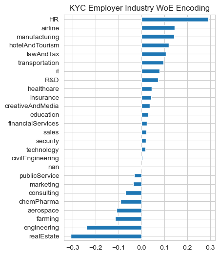
Two insights can be gleaned from this chart. First, the ordering is immediately interpretable without touching the model: HR, airline and manufacturing sit at the positive end, real estate and engineering at the negative end. Second, the whole spread is only about ±0.3, which is a useful reality check: no single industry is a dramatic driver on its own, and I should be sceptical of any story that leans hard on one category.
Why not XGBoost’s native categorical support?
XGBoost 1.6+ handles raw categoricals directly with enable_categorical=True. That would have removed the encoder entirely.
I didn’t because of the goal stated at the top: interpretation. Native categorical splits partition the set of categories, so the feature survives as one column and global SHAP importance still works, but the direction is lost. Category codes have no order, so on a beeswarm plot the colour axis, which encodes low-to-high feature value, means nothing at all. WoE instead gives a numeric column that increases in step with the log-odds of the target, so the colour axis becomes readable: blue is the categories that refer less, magenta the ones that refer more. That, plus the decoded mapping above, is what makesthe extra step worth it for the benefit of explanability (more on that later in the second post of this series).
Combining categories with few observations?
Decision trees don’t inherently struggle with rare categories; the issue is that with very small counts, a split is based on nearly no data, so it’s statistically unreliable and prone to overfitting on noise. When you collapse rare levels into broader buckets, you’re essentially regularizing the model by reducing variance at the cost of some bias. This is usually a good trade.
However, the way you collapse matters. Lumping employer industry in “tourism” and “hotel” together makes domain sense, but purely mechanical approaches (e.g. “combine everything with < 100 samples”) may or may not destroy meaningful signal, depending on whether a rare category is genuinely distinctive.
A middle ground here is target encoding with smoothing, or weight of evidence encoding, which handles rare categories gracefully by borrowing statistical strength from the overall distribution.
Do not use the target variable (Y) to inform your collapsing decisions on the test set! e.g. using a WoE encoding result to collapse non-contributing labels of the entire dataset. This leads us nicely to the next topic: target leakage and the using a pipeline to fight it.
A Pipeline Isn’t Convenience, It’s Leakage Insurance
A Pipeline chains a sequence of transformation steps followed by a final estimator into a single object. When you call pipeline.fit(X_train, y_train), it runs each step’s fit_transform sequentially, passing the output of each step as the input to the next, and finally calls fit on the last step (the model). When you call pipeline.predict(X_test), it runs each step’s transform on the test data (without refitting) before passing the result to the model.
The critical benefit beyond convenience is leakage prevention. Any preprocessing step inside a Pipeline is refitted only on training data within each cross-validation fold, never on validation data. This is the correct behaviour and is easy to get wrong when preprocessing manually outside of a pipeline, especially if you are using techniques such as target encoding and WoE.
Fit the encoder before you cross-validate and the fold has already seen the labels it is about to be tested on.
# -----------------------------------------------
# Build full pipeline
# -----------------------------------------------

pipeline = Pipeline(steps=[
    ('woe', ce.WOEEncoder(cols=woe_features)),
    ('model', XGBClassifier(random_state=42, scale_pos_weight = scale,
                            eval_metric='logloss',
                            objective='binary:logistic'))
])

# -----------------------------------------------
# Define hyperparameter grid
# -----------------------------------------------
param_grid = {
    'woe__regularization': [1.5],
    'model__n_estimators': [100, 200],
    'model__max_depth': [3],
    'model__learning_rate': [0.01, 0.05],
    'model__subsample': [0.8, 0.5],
    'model__colsample_bytree': [0.7, 0.5],
    'model__min_child_weight': [3],
    'model__tree_method': ['hist']
}
As the example code above shows, each step is a tuple of (name, object). The name is arbitrary but must be unique: it’s used to reference that step when setting hyperparameters in GridSearchCV, using the double underscore convention: stepname__parameter.
One thing to note is that encoder hyperparameters can be tuned alongside model hyperparameters within the same search, which is another advantage of keeping everything inside a single pipeline.
What I’d bring to the next model
Reach for the cheap knob before the aggressive one
scale_pos_weightand stratified splits fixed my imbalance without touching the data. Try reweighting before resampling; you can always escalate.Know what the fix costs you
Weighting bought recall and broke probability calibration. Call it out in your report before someone downstream reads a score as a probability.
Convert explicitly, never implicitly
Booleans to ints by hand, ordinal categories in an order you supply. Left alone, an encoder will sort your risk levels alphabetically and you will meet the consequences at the explanation stage.
Pick the encoding that serves the goal
One-hot for a handful of levels, WoE when cardinality grows and you need to explain the model. Had I only wanted predictions, XGBoost’s native categorical support would have been the right call.
Assume leakage is the default
Any transform fitted from the target (WoE, target encoding, even a collapsing decision) leaks unless it lives inside the pipeline and gets refitted per fold.
Tune the encoder and the model together
Once both are in one pipeline, the encoder’s own hyperparameters join the same search. Two things to optimise, one grid.